
Cálculo vectorial para niños
El cálculo vectorial es una parte de las matemáticas que estudia los vectores en espacios con dos o más dimensiones. Es muy útil para entender y resolver problemas en la ingeniería y la física.
En el cálculo vectorial, trabajamos con dos tipos principales de "campos":
- Los campos vectoriales asignan un vector (que tiene dirección y magnitud) a cada punto en el espacio. Por ejemplo, el flujo del agua en una piscina es un campo vectorial, porque en cada punto el agua se mueve en una dirección y con una velocidad.
- Los campos escalares asignan un número (un valor escalar) a cada punto en el espacio. Por ejemplo, la temperatura de una piscina es un campo escalar, ya que en cada punto hay un valor de temperatura.
Cuatro operaciones son muy importantes en el cálculo vectorial:
Contenido
¿Qué es el Cálculo Vectorial?
El cálculo vectorial nos ayuda a entender cómo cambian las cosas en el espacio. Imagina que quieres saber cómo se mueve el aire alrededor de un avión o cómo se distribuye el calor en una habitación. Para eso, usamos el cálculo vectorial.
Campos Escalares y Campos Vectoriales
Para entender el cálculo vectorial, primero necesitamos saber qué son los campos.
- Campos escalares: Piensa en la temperatura de una habitación. En cada punto de la habitación, hay un número que representa la temperatura. Ese es un campo escalar. Otros ejemplos son la presión o la densidad.
- Campos vectoriales: Ahora, imagina el viento. En cada punto del aire, el viento tiene una dirección y una fuerza. Eso es un campo vectorial. Otros ejemplos son la velocidad del agua en un río o la fuerza de la gravedad.
Operaciones Clave en el Cálculo Vectorial
El cálculo vectorial tiene herramientas especiales para analizar estos campos. Las más importantes son:
Gradiente: ¿Cómo cambia una propiedad?
El Gradiente nos dice qué tan rápido cambia un campo escalar y en qué dirección. Por ejemplo, si estás en una montaña y quieres saber la dirección más empinada para subir, el gradiente te lo diría. El resultado de un gradiente es un campo vectorial.
Rotor: ¿Hay giro en un campo?
El Rotor (o rotacional) mide si un campo vectorial tiende a girar alrededor de un punto. Imagina un remolino en el agua; el rotor nos diría qué tan fuerte es ese giro. El resultado de un rotor es otro campo vectorial.
Divergencia: ¿Se dispersa o se concentra algo?
La Divergencia mide si un campo vectorial tiende a "salir" o "entrar" en un punto. Por ejemplo, si tienes una manguera de agua, la divergencia sería alta en la boquilla porque el agua se dispersa. Si el agua se concentra en un sumidero, la divergencia sería negativa. El resultado de una divergencia es un campo escalar.
Laplaciano: ¿Cómo se relaciona el promedio?
El Laplaciano es una operación más avanzada que combina el gradiente y la divergencia. Nos ayuda a entender cómo se distribuye una propiedad en el espacio, relacionando el valor de una propiedad en un punto con el promedio de sus valores alrededor.
Historia del Cálculo Vectorial
El estudio de los vectores comenzó con las ideas de William Rowan Hamilton, un matemático que inventó algo llamado "cuaterniones". Los cuaterniones eran una forma de representar números que tenían una parte escalar y una parte vectorial, y se usaban para explorar el espacio físico.
Sin embargo, los cuaterniones eran un poco complicados de usar. Los científicos se dieron cuenta de que muchos problemas se podían resolver si se trabajaba solo con la parte vectorial por separado. Así fue como nació el "Análisis Vectorial".
Gran parte de este trabajo se lo debemos a dos físicos: el estadounidense Josiah Willard Gibbs (1839-1903) y el inglés Oliver Heaviside (1850-1925). Ellos simplificaron las ideas y las hicieron más fáciles de aplicar en la física y la ingeniería.
Aplicaciones del Cálculo Vectorial
El cálculo vectorial se usa en muchas áreas, especialmente para entender cómo se comportan las funciones en varias dimensiones.
Encontrar Puntos Especiales en Campos Escalares
Una aplicación importante es encontrar los puntos más altos, los más bajos o los puntos de "silla de montar" en un campo escalar.
Máximos y Mínimos: Puntos Altos y Bajos
- Un máximo es como la cima de una montaña: es el punto más alto en una región.
- Un mínimo es como el fondo de un valle: es el punto más bajo en una región.
Puntos de Ensilladura: Ni Máximo ni Mínimo
Un punto de ensilladura es un punto donde la función no es ni un máximo ni un mínimo. Imagina una silla de montar a caballo: en una dirección subes, pero en otra bajas.

Para encontrar estos puntos, los matemáticos usan herramientas del cálculo vectorial, como las derivadas parciales y la matriz hessiana, que les ayudan a analizar la forma de la función en esos puntos.
Galería de imágenes
-
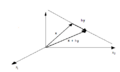
Representación de una derivada direccional.

Véase también
 En inglés: Vector calculus Facts for Kids
- Cálculo de matrices
- Integral de línea
- Integral de superficie
- Integral múltiple
- Multiplicadores de Lagrange
- 1-forma
- coordenadas ortogonales
- dual de Hodge
- electrostática
- magnetostática
- operador nabla
- teorema de la divergencia
- teorema de Green
- teorema de Stokes
